Synposis
The claims of antenna manufacturers are not to be trusted. Therefore, to have a good grasp on the network’s RF behavior, we need to analyze and characterize the antennas that are to be used for HamWAN purposes. The spectrum of interest is listed in the Spectrum Allocation page. 5.25GHz - 5.925GHz with a “don’t care” gap between 5.35GHz - 5.47GHz.
Signal Generation
For the purposes of measuring, the 8660C sweeping signal generator will be used along with a frequency tripler and amplifier. Sweeps should exceed the measurement band by at least 25MHz to allow for signal settling. Therefore, sweeps will be between 5.225GHz and 5.95GHz. The center frequency is then 5.5875GHz. On the 1/3rd frequency sweeper this becomes 1.8625GHz. The sweep width to be configured is 241.666…MHz. The input level to the frequency tripler should be about +10dBm, so this needs to be set on the 8660C. Between the tripler loss and the amplifier gain, the resulting tripled signal should be just slightly less than the input power level. +4dBm to +6dBm are typical output level values.
Level Error Correction
During the sweep, the 8660C signal generator, the tripler, the amplifier and the interconnects will all change the level of the signal with frequency. This antenna input power variance needs to be accounted for and subtracted from the measurement.
Sample Antenna Coupling Measurement
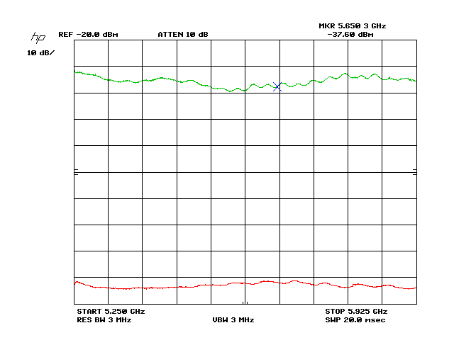
The above graph shows a sample antenna power transfer measurement from an ARC Wireless ARC-VS5818SD1 to a Laird SAH58-120-16-WB over an approximate distance of 6.5ft. TX power was about +4dBm @ the center frequency, and the error in the TX power level can be seen in the lower trace. This trace has been level-shifted so its absolute values are incorrect, but the relative level relationships between peaks and valleys are correctly scaled. The top trace shows the power at the RX antenna, with the amplitude corrected for TX power variations. A marker shows the approximate start of the amateur band. It is high by 300kHz due to the resolution of the instrument and the large span here. The approximate path loss at the marker is 40dB. The antennas were not perfectly aligned for this test.
Due to the measurement technique the top trace therefore shows the combined gain variations of the TX and RX antennas, assuming the free space between them to have a constant loss over the frequency span. This is useful information, but cannot pin point the exact behavior of each antenna so that they can be compared.
Reference Antenna
A third antenna is needed with a known gain error over the frequency band of interest for at least one direction of radiation. This antenna’s error can then be combined with the TX power level error and will result in an error corrected emitted field strength for the RX antenna to consume. To minimize multipath interference a 21dBi directional parabolic antenna will be used, the Laird GD5W-21P. This antenna still has a reasonable beamwidth of 10 degrees. Any future measured antennas must have all their radiating elements well within this degree beamwidth of the reference antenna.
In order to determine the reference antenna gain characteristic two of them will be used in a coupling measurement. This makes the assumption that manufacturing variations are minimal and that both antennas will have the same behavior. The received signal (corrected for power variations) will be composed of an assumed constant free space loss, and exactly twice the gain error of the reference antenna model since it’s used for both TX and RX. This error curve can then be divided by two to obtain the exact gain error characteristic of the reference antenna.
Regular spectrum analyzer techniques of “MAX HOLD” and “A-B->A” can be used for the majority of the steps described above, but taking the existing error curve of the signal generator and further correcting it with 1/2 of the coupling error is not something the 8566A can do. Therefore, I have written some crude software to be used at the point of the process where the signal generator curve is stored in trace B and the sig-gen-corrected antenna coupling curve is stored in trace A. It is attached to this page and can be downloaded at the bottom. Look for “MergeCorrectionCurves.py”.
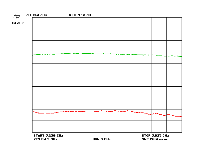
Below is the coupling curve (top trace) between the two reference antennas with just signal generator correction applied:

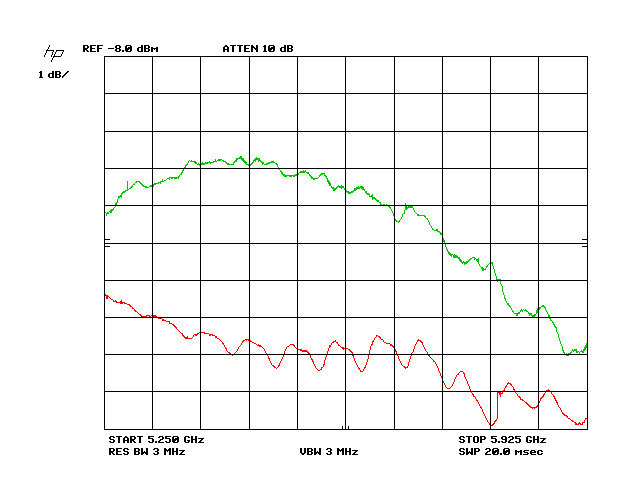
And here is the coupling curve (top trace) between the two reference antennas with signal generator + radiating antenna strength corrected:
You can see the extent of variability in that top trace has dropped by half, just as expected. This means we now have an error-corrected radiated electromagnetic field strength. If this bottom correction curve is uploaded to the spectrum analyzer, and a measurement made with any other receive antenna, the resulting top trace will be the exact error of the DUT antenna alone.
For anyone curious, the single antenna correction data is as follows:
MergeCorrectionCurves.py execution snippet
Transforming Trace A data into mean-offset correction values...
1,2,2,1,-1,-3,-3,-3,0,-3,-3,-3,-4,-3,-3,-3,-2,-3,-1,-2,-1,-2,-2,-1,0,-1,1,0,0,0,0,1,0,1,0,0,0,0,0,1,-1,-1,0,-1,-1,0,-1,1,0,1,0,0,1,1
,1,1,2,1,3,2,2,2,4,2,4,3,5,3,2,4,2,4,2,4,2,2,3,3,2,3,3,2,3,3,3,3,3,5,3,5,3,4,4,3,3,4,3,3,4,3,5,3,2,4,3,4,3,4,3,2,3,3,2,3,4,2,4,3,5,3
,3,4,3,4,3,3,4,3,3,3,7,4,3,3,3,2,2,2,2,2,3,2,3,2,4,2,4,2,3,2,4,3,3,3,3,3,5,4,6,4,6,4,6,5,5,5,5,5,5,6,5,8,5,5,7,5,6,5,5,5,5,6,5,7,6,8
,5,7,6,7,5,6,7,6,7,7,7,8,7,9,7,9,7,8,7,8,7,8,7,7,7,9,7,9,7,9,7,9,7,8,7,7,7,7,8,7,6,9,7,8,7,8,7,8,7,7,7,7,7,7,9,7,9,7,7,9,7,8,6,7,6,6
,7,6,7,6,8,6,8,6,8,6,6,7,6,7,6,7,7,6,8,7,8,6,8,7,8,7,6,8,7,7,6,7,7,7,8,6,8,6,8,7,9,7,8,7,7,8,7,8,7,8,7,7,9,7,9,7,9,7,9,7,8,6,7,7,7,7
,7,6,8,6,9,6,8,6,7,6,7,6,7,7,7,7,8,7,10,7,9,8,8,8,8,8,8,8,8,9,8,8,10,8,10,8,9,8,8,8,8,8,8,8,7,10,8,9,7,7,8,7,8,7,7,9,8,9,7,9,7,9,7,9
,8,8,7,9,7,9,7,9,7,9,7,9,7,8,7,8,7,7,8,7,8,7,7,8,7,8,7,8,6,6,7,7,7,7,8,6,9,6,6,7,6,6,5,5,5,5,6,5,7,5,8,5,7,5,7,6,6,7,6,6,6,6,7,7,8,6
,8,6,8,6,7,6,7,5,6,5,6,5,6,5,7,5,7,5,6,5,7,5,6,6,5,6,6,6,7,6,7,6,8,6,8,6,8,7,7,6,7,6,6,6,6,7,7,5,8,5,7,5,7,5,6,5,6,5,5,6,5,5,6,5,7,5
,7,6,7,6,7,6,6,6,6,6,6,8,5,5,8,6,8,5,6,5,5,5,5,5,4,6,4,6,4,3,5,4,4,3,4,5,3,6,3,5,4,5,3,4,4,4,3,3,3,5,3,5,3,5,3,4,3,4,3,3,5,4,5,4,6,4
,4,5,4,4,4,4,4,3,4,3,5,3,4,3,3,2,3,2,2,2,2,2,3,1,3,2,4,2,4,2,3,2,3,2,2,3,2,3,3,3,3,3,3,3,3,3,3,3,3,2,2,3,2,2,2,2,2,2,2,1,2,1,1,2,1,1
,1,2,1,3,2,2,3,2,3,2,3,3,3,3,3,3,2,3,2,2,2,2,2,2,1,2,1,1,1,1,0,0,0,0,0,0,0,0,0,1,0,1,0,1,1,1,1,1,1,1,0,1,0,0,-1,0,-1,-1,-1,-1,-2,-2,
-2,-2,-2,-3,-3,-3,-3,-3,-3,-3,-3,-2,-3,-3,-3,-3,-3,-3,-4,-3,-3,-3,-4,-4,-4,-4,-4,-4,-4,-5,-4,-4,-4,-5,-4,-4,-4,-4,-4,-4,-4,-4,-4,-4,
-3,-3,-3,-3,-3,-3,-4,-3,-3,-4,-3,-3,-4,-4,-4,-4,-4,-5,-5,-5,-5,-6,-5,-5,-6,-6,-6,-6,-6,-6,-6,-6,-6,-6,-6,-5,-6,-5,-5,-3,-5,-3,-4,-3,
-4,-4,-4,-4,-4,-4,-4,-4,-4,-4,-5,-4,-5,-3,-5,-4,-6,-4,-6,-6,-6,-6,-6,-6,-6,-6,-7,-6,-5,-7,-6,-7,-7,-7,-6,-7,-6,-6,-6,-6,-6,-6,-6,-6,
-6,-7,-7,-7,-8,-6,-8,-8,-9,-9,-9,-9,-10,-10,-10,-10,-10,-11,-10,-10,-10,-11,-10,-11,-11,-10,-11,-11,-11,-12,-12,-12,-13,-13,-14,-13,
-14,-14,-14,-15,-14,-15,-15,-16,-16,-15,-16,-15,-15,-15,-15,-16,-15,-14,-15,-15,-15,-15,-13,-15,-14,-14,-14,-14,-14,-14,-14,-15,-15,
-14,-15,-15,-13,-15,-13,-15,-14,-15,-14,-13,-15,-13,-13,-14,-13,-13,-13,-13,-11,-13,-11,-13,-12,-13,-12,-12,-12,-12,-11,-12,-10,-12,
-12,-12,-12,-12,-12,-13,-13,-14,-13,-13,-14,-13,-12,-14,-12,-14,-12,-15,-15,-14,-14,-14,-13,-13,-13,-11,-13,-13,-11,-13,-11,-13,-12,
-13,-14,-14,-13,-14,-14,-13,-15,-13,-15,-14,-16,-16,-16,-17,-17,-17,-17,-17,-17,-17,-17,-16,-17,-15,-17
The units are in HP’s custom “O2” data scale. No relationship was derived between O2 and dB since it was not needed to properly correct the response here. The actual dB corrections are visible in the graphs above. This data set belongs to the antenna and it is valid to re-use it with the antenna connected to a different signal source. It is however only valid over the exact frequency span of 5.25GHz - 5.925GHz.
Improved Measurement Precision
Antenna beamwidths and frequency ranges are specified at -3dB power points. Using a 10dB/graticule system makes it very hard to see when 3dB has been crossed. The problem with using 1dB/ mode is that you only get 10dB of dynamic range on your measurements. The measurements of signal source error are done at much higher power levels than the measurements of antennas over the air. The difference in levels between these two measures is much larger than 10dB, so it would seem 1dB/ mode is incompatible with this wide dynamic range of measurement. However, the internal design of the 8566A spectrum analyzer stores correction trace data in screen pixel memory, not in absolute dB values. This means that the reference level of the analyzer can be shifted between signal generator and antenna measurements, and the math will still be correct. The only restrictions are that the dB/graticule stay constant between measurements and each measurement, on its own, not span more than 10dB of signal range. Below is a result in 1dB/ precision mode:
The bottom trace is the error of the signal source, and the top trace is the combined error of 2 21dBi grid antennas. Using this improved technique it is possible to measure a higher precision reference antenna correction curve:
MergeCorrectionCurves.py execution snippet
Transforming Trace A data into mean-offset correction values...
9,9,8,8,6,8,9,10,9,10,10,9,10,10,10,11,11,12,11,13,13,15,15,17,19,19,21,21,23,27,29,28,29,29,31,28,33,35,34,35,35,36,36,
37,37,37,37,37,50,38,39,39,40,40,40,42,42,43,43,45,45,46,46,48,48,49,49,49,49,50,50,49,49,48,48,48,48,47,46,46,44,45,44,
43,43,43,43,43,43,42,43,43,42,43,44,44,44,44,44,44,45,44,46,46,47,46,46,47,48,47,47,47,48,48,48,48,49,48,50,49,50,52,50,
50,51,51,51,51,52,52,53,53,53,53,54,54,54,55,54,54,54,54,54,55,55,55,54,54,55,55,55,55,56,56,56,58,59,60,59,61,62,64,65,
65,66,67,69,70,72,73,74,75,77,76,78,80,79,79,80,78,80,79,80,79,79,78,77,77,77,78,78,76,76,74,76,74,76,72,74,74,74,74,75,
75,74,74,75,74,76,75,77,76,76,76,76,77,76,78,77,76,77,76,77,76,78,76,79,78,78,78,78,80,78,79,80,80,81,80,80,80,81,81,81,
81,81,80,80,80,79,79,78,78,77,76,77,76,76,75,76,74,76,75,76,75,75,76,75,76,77,78,78,78,79,79,81,82,82,81,84,83,81,82,82,
83,82,82,81,80,80,79,78,77,76,74,74,75,73,72,72,73,72,72,72,73,74,73,75,75,77,76,78,79,78,79,80,80,81,80,81,80,80,79,80,
78,78,78,76,76,76,76,74,75,74,75,73,75,74,75,75,76,76,76,76,77,77,77,76,78,78,78,76,77,76,77,76,74,75,74,73,71,70,69,69,
67,65,64,63,63,62,61,61,60,59,59,59,58,58,59,59,58,58,60,58,58,59,58,59,58,58,59,59,58,58,57,59,59,59,60,59,60,61,62,63,
61,63,62,64,64,64,63,65,65,65,65,65,64,65,64,63,63,64,61,61,61,59,59,58,58,57,56,56,55,55,55,55,56,60,61,55,55,54,56,56,
58,57,58,58,59,61,62,61,62,62,61,60,62,59,60,57,58,56,57,53,52,52,51,49,46,48,45,44,44,41,43,40,41,39,41,40,41,42,43,42,
44,44,45,44,43,44,45,43,45,42,44,41,42,42,42,40,39,40,38,38,37,37,36,37,37,34,37,34,37,36,38,38,39,38,40,40,39,41,40,42,
43,41,43,41,45,42,43,44,43,44,43,43,43,42,41,41,38,40,38,36,36,37,33,36,33,35,31,33,30,32,30,32,32,27,29,29,29,29,26,28,
26,26,24,26,26,23,24,22,22,20,20,20,20,20,18,19,18,19,19,18,18,19,18,18,18,17,17,16,16,15,14,13,13,10,9,7,6,4,3,0,1,-2,0
,-3,-1,0,-4,-2,-3,1,1,-1,2,1,6,4,8,7,10,9,13,19,14,14,14,15,16,14,16,14,16,14,16,16,14,16,15,13,13,9,11,8,8,6,6,5,4,5,4,
4,4,4,4,3,4,4,4,4,3,4,3,2,2,2,0,-1,0,-2,-3,-4,-6,-6,-7,-9,-9,-13,-12,-15,-14,-15,-15,-17,-16,-17,-16,-15,-17,-17,-16,-18
,-17,-19,-18,-21,-19,-21,-22,-24,-26,-27,-31,-29,-31,-36,-35,-40,-39,-44,-42,-47,-45,-49,-46,-49,-48,-49,-50,-49,-49,-49
,-50,-51,-49,-51,-50,-52,-50,-52,-51,-51,-53,-53,-56,-53,-58,-55,-59,-57,-59,-61,-58,-58,-62,-59,-61,-59,-61,-58,-61,-58
,-60,-56,-58,-56,-55,-54,-55,-54,-53,-52,-52,-53,-50,-53,-50,-50,-51,-55,-53,-58,-55,-54,-57,-60,-61,-63,-63,-64,-65,-66
,-67,-67,-68,-70,-68,-69,-68,-68,-67,-65,-65,-63,-63,-62,-60,-61,-60,-59,-59,-60,-60,-61,-63,-65,-67,-69,-71,-74,-76,-79
,-81,-85,-83,-83,-83,-83,-82,-83,-86,-87,-90,-91,-97,-99,-98,-103,-105,-108,-109,-110,-113,-113,-113,-114,-116,-115,-117
,-117,-118,-118,-121,-122,-121,-125,-123,-123,-127,-126,-126,-128,-128,-128,-128,-130,-126,-128,-126,-126,-124,-124,-122
,-122,-123,-122,-121,-122,-121,-121,-123,-121,-124,-122,-125,-122,-125,-124,-124,-124,-125,-126,-125,-126,-127,-128,-126
,-130,-128,-128,-127,-127,-128,-127,-127,-123,-121,-123,-121,-121,-117,-119,-116,-117,-114,-116,-117,-115,-118,-115,-118
,-117,-120,-120,-123,-122,-125,-125,-126,-125,-127,-128,-130,-131,-136,-135,-135,-136,-138,-139,-139,-143,-140,-147,-144
,-147,-147,-151,-152,-154,-156,-159,-161,-163,-166,-167,-169,-170,-171,-173,-175,-176,-177,-178,-178,-179,-178,-180,-178
,-180,-179,-180,-179,-178,-178,-177,-176,-178,-174,-176,-174,-176,-173,-173,-174,-172,-173,-170,-175,-172,-173,-174,-174
,-176,-174,-177,-171,-172,-175,-171,-175,-171,-169,-168,-167,-168,-167,-166,-161,-163
The resulting high precision frequency response curve for one of these 21dBi grid antennas looks like this:
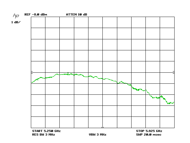
A much clearer view than before! The antenna is within a 3dB range throughout the entire spectrum of interest. The error correction trace has been removed for clarity, since it’s so large in range that it actually crosses the antenna characteristic trace.
Radiation Pattern Measurement
Frequency response is only part of the story. Another very important aspect of any antenna is its radiation pattern. It is rather difficult to measure this correctly, and usually requires an anechoic chamber, which is prohibitively expensive. In this cost-optimized implementation the anechoic chamber is provided by the great outdoors. A flat field with no objects around and no detectable RF sources at the measurement frequency is ideal. The other expensive part of full 3D radiation pattern measurement is the DUT antenna positioning system. It has to angle the antenna just right to take readings. In this cost-optimized implementation, the angular positioning is restricted to 1 axis at a time, allowing for just circular sweeps. The angular positioning is approximated by using a synchronous motor based rotor system, fed by a fixed frequency (60Hz wall power). The time for one full rotation is first measured (64 seconds in my case) and then given to the software. The measurement software and the rotation have to be started at the exact same time by manual action. No fancy computer control here.
After a full set of readings is taken the software counts the number of data samples it was able to obtain during the specified time period of assumed 360 degree rotation, and computes the angular resolution per sample (~0.5deg in my case). It then scans the whole data set to find the largest magnitude reading. These are in dBm as they arrive from the spectrum analyzer. All the readings are then offset by the negation of this maximal reading so as to normalize the dataset at peak magnitude = 0dB. Next, an algorithm sweeps the angular magnitude data once more to identify the -3dB power points around the peak. The angular difference between these points is reported as the antenna’s beamwidth. The center angle of the beamwidth is computed based upon the angular position of the -3dB points, and the whole data set is rotated so that the beamwidth center is at 0 degrees. After this normalizing rotation, a couple magnitude samples are taken at -120 degree and +120 degree angles. These angles correspond to the directions of radiation from co-located sector antennas and it’s important that the attenuation at these angles is high to reduce interference between the sectors. Finally the dataset is converted into R-code which defines a polar plot using the plotrix R library.
The code for doing all of this is attached to this page in the file “RadiationPattern.py”.
Lab Procedure - Frequency Response Setup
- Power up 8566A
- Set Ref Level to +30dBm, Start Freq = 5.25GHz, Stop Freq = 5.925GHz, 10dB/
- Power up 8660C
- Enter 1.8625GHz Center Frequency into 8660C
- Enter 241.666666MHz Sweep Width into 8660C
- Set sweep mode to off
- Apply +5VDC power to MiniCircuits amplifier (post-tripler). Should read 60mA.
- Set output of 8660C to 10dBm
- Using the exact coax cables that will be attached to the ref antennas, connect their ends with an N(F)-N(F) coupler.
- Observe signal on 8566A and adjust Ref Level until signal is nearly full scale and not clipping
- Adjust dB/ and Ref Level until 1dB/ is achieved and the centered frequency signal (no sweeps) is about 50% amplitude on screen
- Set Sweep Mode to “Auto” on 8660C, and make sure Rate is set to Slo
- Enable Max Hold on 8566A and make sure no part of the sweep is clipped on bottom or top
- Try to align the peak of the max-held sweep trace with the top of the graticules without clipping (adjust Ref Level)
- With everything levelled properly, press Clear-Write on 8566A and then Max Hold again.
- Allow for 2-3 passes so that the line is smoothed out.
- On 8566A, press “A <-> B”
- Press “Enter” under “Display Line” section.
- Move the display line so that it is just below the bottom point of the A trace, but not touching it.
- Press”B - DL -> B”
- The signal source and interconnect errors are now stored in B.
- Press “Off” under “Display Line” section.
- Turn Sweep Mode to “Off” on the 8660C
- Set trace A to Clear-Write mode on the 8566A. You should see the centered frequency being displayed.
- Remove the N(F)-N(F) coupler between the coax lines and attach the pair of reference antennas.
- Adjust “Ref Level” on 8566A until signal is in the middle of the screen.
- Do fine-alignment of the reference antennas to maximize signal on 8566A
- Once satisfied, adjust Ref Level to once again put the signal level in the middle of the screen
- Set Sweep Mode to “Auto” on the 8660C
- Press “Max Hold” on the A trace on the 8566A
- Observe a full sweep to determine max/min levels.
- Adjust Ref Level so that the “Max Hold” trace is as high up as possible on the screen without clipping.
- Make sure bottom is not clipping either. If it is, 1dB/ mode will not work and 2dB/ needs to be tried by restarting the whole procedure.
- With the well-bounded trace configured, enable “A - B -> A” mode on the 8566A
- Hit Clear-Write and Max Hold to restart the max holding in error-correcting mode now
- Allow for 2-3 sweeps, or enough to eliminate any noise in the trace
- Run the MergeCorrectionCurves.py script to adjust the B trace correction curve for the error found in the reference antennas
- Hit LCL to regain local control of the 8566A instrument
- Hit Clear-Write and Max Hold again on Trace A to measure the Frequency Response of one of the reference antennas now
- Allow 2-3 sweeps to clear up the trace before printing
- Disconnect the RX reference antenna and remove from mount in preperation for other antennas to be measured
Lab Procedure - Frequency Response of Subsequent Antennas
- As a safety measure, increase the Reference Level on the 8566A sufficiently so that the new DUT antenna will not cause clipping
- Disable “A - B -> A” mode on the 8566A
- Press Clear-Write to disable Max Hold mode on Trace A
- Mount and connect the new DUT antenna
- Set Sweep Mode to “Off” on the 8660C
- Adjust Ref Level on 8566A until signal is mid-way up the screen
- Align the new DUT RX antenna so as to maximize signal reading
- Adjust Ref Level on 8566A until signal is mid-way up the screen again
- Set Sweep Mode to “Auto” on 8660C
- Press Max Hold on Trace A on 8566A
- Adjust Ref Level of 8566A so as to maximize measured amplitude without clipping at top or bottom
- Once the level is good enable “A - B -> A” mode
- Press Clear-Write and Max Hold again to restart the measure, for real this time
- Allow 2-3 passes to smooth out the measurement trace
- Print/record results
- Disconnect and dismount the just-measured antenna